
Curt Trig
Table of Contents
1 Introduction
Precise trigonometry is critical, needless to say, if the objective of safely landing on and returning from the Moon is to be met.
In 2019, on the 50-year anniversary of the Apollo 11 flight, the source code for both the Lunar Module's (LM) Apollo Guidance Computer (AGC) and the Command Module's (CM) AGC were released into the public domain. In both repositories, CM's Comanche055, dated Apr. 1, 1969, and LM's Luminary099, dated July 14, 1969, circular functions are coded in the same remarkably brief source file, SINGLE_PRECISION_SUBROUTINES.agc 1.
The concise code, to the point of curtness, implements both functions \(sin(\pi x)\) and \(cos(\pi x)\) in only 35 lines of assembly!
The rare combination of brevity and extreme accuracy is the result of a long history of mathematical research on the classical problem of best approximation. As for trigonometric, or in this instance circular functions their numerical computation is an even older problem dating back to the first Mayan and Greek astronomers.
The best approximation of a continuous function by a limited degree polynomial was studied from the second half of the 19th century, once basic notions in calculus were firmly grounded Pachéon2009.
A second wave of applied research can be dated back to the 1950s and 1960s when the generalized use of computers for scientific calculations prevailed. The focus of these applied numerical algorithms was often a converging process towards the best approximation, based on further developments of the early theoretical 19th-century research, an idea originally published in 1934 Remez1934:2. The period saw the development of a deeper understanding of the approximation theory and a flurry of variations for its practical computer implementation.
These developments, in turn, became a fundamental tool in the study of digital signal processing in the 1970s, when introduced in the context of filter design Parks1972.
Most of today's practical implementations date mainly to that era. And the "Moon Polynomial", at the core of the intense 35 lines of code in Comanche and Luminary, is a wonderful tribute to the engineering of the times.
2 First Polynomial on the Moon
As a starting point, and armed with the modern programming language Python (v. 3.8) together with its fundamental calculation package NumPy (v. 1.18.1 for this paper), we embark on a naive rewrite of this single precision circular sine function from 1969. The quick effort satisfactorily produces the following graph, which compares the approximation polynomial used in the Apollo code against the sine function on the range \([-\pi, \pi]\) (curtesy of NumPy).
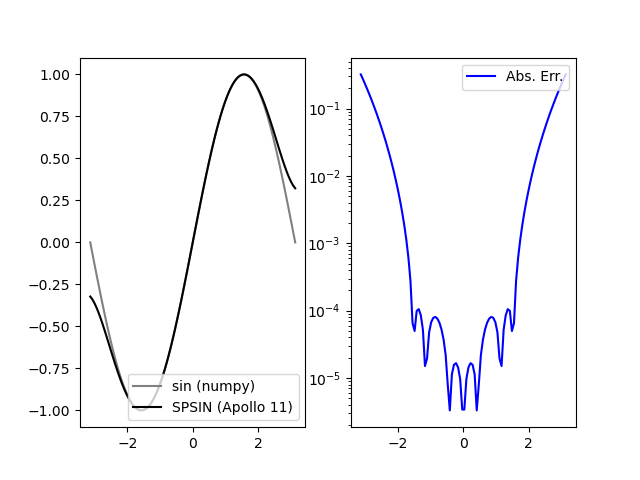
The sine function as implemented in the Apollo 11 Guidance Computer. Left: double precision sine function from NumPy and SPSIN from AGC code; Right: Absolute error plotted on a logarithmic scale
Several points of interests are apparent in the venerable implementation. The maximum absolute error over the whole \([-\pi, \pi]\) range is \(0.32214\), but the minimum is \(3.30701\:10^{-6}\) which is certainly an achievement for so brief a source code. Apparently the floating point representation on the AGC did not use the traditional mantissa and exponent, as usually found in high-precision mathematical libraries since, but only a simpler fractional representation relying instead on the extra-careful programming of argument reduction to handle magnitude. (The AGC had a total of 38K words of memory, beginning with 2K 16-bit words of read/write memory and 36K of read-only storage, so that restricted memory resources were another constraint AGC2010.)
The plot on the right also illustrates a "wing" pattern in the absolute errror, where the extrema increase as \(x\) approaches the limits of the range of the approximation. This is something we will find again and again in our incursions into approximation theory and its implementations.
Indeed, it is now known that when approximating a function from its values \(f(x_i)\) at a set of evenly spaced points \(x_i\) through $(N+1)$-point polynomial interpolation often fails because of divergence near the endpoints: the "Runge Phenomenon" named after Carl David Tolmé Runge (1856-1927). This could suggest that the polynomial used in the AGC implementation to approximate the sine function may have been computed from evaluations on evenly spaced points. The use of an evenly spaced points range is uncommon nowadays for reasons that will be brushed on in the next section, but this simple observation adds to the mystery of the origin of the first polynomial that made it to the Moon.
In its SPSIN function, the AGC code computes, after doubling the argument, the following approximation:
\begin{equation} \frac{1}{2} \sin (\frac{\pi}{2}x) \approx 0.7853134 x - 0.3216147 x^3 + 0.0363551 x^5 \end{equation}As explained by Luis Batalha and Roger K., in their informed review of the AGC code, these terms are close to the terms of the Taylor approximation, but not exactly identical. This particular polynomial was most certainly preferred over the truncated Taylor series as it provide smaller error in the interval of interest. The commentators indeed discovered that the polynomial approximation used here can be found in a 1955 Rand Corp. report Hastings:1955 by Cecil Hastings, Jr., assisted by Jeanne T. Hayward and James P. Wong, Jr.: Approximations for Digital Computers, on p. 138 (Sheet 14 of Part 2):
\begin{equation} \sin (\frac{\pi}{2}x) \approx 1.5706268 x - 0.6432292 x^3 + 0.0727102 x^5 \end{equation}the exact same polynomial (when coefficients are doubled).
3 Introductory mathematical background for the Moon Polynomial
3.1 Best approximation
In the well-studied mathematical problem of best approximation, a continuous real function \(f\) on an interval \(I=[a,b]\) is given and we seek a polynomial \(p^*\) in the space \(\mathcal{P}_n\) of polynomials of degree \(n\) such that:
\begin{equation} \| f - p^* \| \leq \| f - p \|,\: \forall p \in \mathcal{P}_n \end{equation}where \(\| . \|\) is the supremum norm on \(I\)2.
The approximation problem consists then of three major components:
- The function \(f\) to approximate usually picked up from a function class \(\mathcal{F}\) endowed with particular properties, here real functions of the real variable over the given interval \(I\).
- The type of approximation sought, usually polynomials but also rational functions and continued fractions according to the problem at hand3.
- The nature of the norm. Popular standard choices are the supremum, or uniform or \(L_{\infty}\), norm as above, in which case the approximation is called the minimax polynomial; the (weighted) least-squares or \(L_2\) norm defined by \(\| g(x) \|_2 = ( \int_{I} g^2(x) w(x) dx )^{ \frac{1}{2} }\) where \(w\) is a positive weight function.
In the construction of approximate polynomials several types of errors conspire to divert progresses: interpolation errors (how large \(f(x) - p(x)\)?), argument reduction errors (in the mapping of original arguments to \(f\) into the approximation interval \(I\)), and rounding errors both in representing constants like \(\pi\) and computing sums, products and divisions.
Furthermore there are relatedly several notions of best approximations:
- A polynomial \(p\) is an \(\varepsilon\) good approximation when \(\| f - p \| \leq \varepsilon\) ;
- A best polynomial \(p^*\) is such that \(\| f - p^* \| \leq \| f - p \|, \: \forall p \in \mathcal{P}_n\) ;
- A near-best polynomial \(p\) within relative distance \(\rho\) is such that \(\| f - p \| \leq (1 + \rho)\| f - p^* \|\)
In practice all three types of approximations play a role in the construction of polynomials.
3.2 Taylor Series
A first practical idea is to look at the Taylor (after Brook Taylor FRS, 1685-1731) series representation of \(\sin (x)\) and truncate it to the degree we are interested in:
\begin{equation} \sin (x) = \sum_{0}^{\infty} \frac{(-1)^k}{(2 k + 1)!} x^{2 k + 1} \end{equation}which, since it is being taken at \(x=0\), is in fact named a MacLaurin series (after Colin Maclaurin, 1698-1746).
Calculation the Maclaurin series for the target function in the Apollo 11 code using the NumPy.polynomial results in:
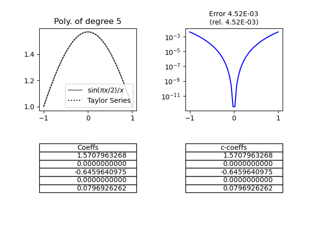
Truncated (to \(k=2\)) Taylor (Maclaurin) series approximation of \(sin(\frac{\pi}{2} x)/x\) computed on equally spaced points over the range \([-1,1]\). Top left: function and its approximation; Top right: absolute error; Bottom: approximation polynomial coefficients; left on the polynomial basis, right on the monomial basis, identical for Taylor series.
Even on the quick truncation of the Maclaurin series (\(k=2\)), it is apparent that the approximation polynomial has a large absolute error on the whole interval \(I\). As readily seen, the precision is however much better on a restricted interval \([-\varepsilon, \varepsilon]\) around 0 – in fact, down to the smallest double-precision floating point in the machine representation. And while double-precision libraries often use minimax of Chebyshev polynomials – to be discussed below – which require somewhat fewer terms than Taylor/Maclaurin series for equivalent precision, Taylor series are superior at high-precision since they provide faster evaluation Johansson2015. Hence a sophisticated argument reduction can balance the lack of accuracy of the truncated Maclaurin series on the larger interval within the bounds of a given time/precision compromise.
3.3 Newton's Method of Divided Differences
The generalization of the linear interpolation to a set of points where the interval difference is not the same for all sequence of values is known as the Newton's method of divided differences. Its computer implementation is made simple by the iterative nature of the calculations and their natural layout in tabular form.
Provided a trial reference, a set of \(n+1\) distinct points of \(I\) with the evaluation of \(f\) at these points, \(x_i, \:y_i=f(x_i) \: i=0,1,...n\), Newton's formula:
\begin{equation} p(x) = y_0 + (x - x_0)\delta y + (x - x_0)(x - x_1)\delta^2 y + ... + (x - x_0)(x - x_1)...(x - x_{n-1})\delta^n y \end{equation}ensures that the polynomial of degree \(n\) passing through all the trial reference points is unique. In the formula, the \(\delta^k y\) are called the divided differences and defined by recurrence:
\begin{equation} \delta y[x_i, x_j] = \frac{y_j - y_i}{x_j - x_i}, \: \delta y = \delta y[x_0,x_1] \end{equation} \begin{equation} \delta^2 y[x_i, x_j, x_k] = \frac{\delta y[x_j, x_k] - \delta y [x_i, x_j]}{x_k - x_i}, \: \delta^2 y = \delta^2 y [x_0, x_1, x_2] \end{equation}…
\begin{equation} \delta^n y[x_{i_0}, x_{i_1}, ... , x_{i_n}] = \frac{\delta^{n-1} y[x_{i_1}, x_{i_2}, ... , x_{i_n}] - \delta^{n-1} y [x_{i_0}, x_{i_1}, ... , x_{i_{n-1}}]}{x_{i_n} - x_{i_0}}, \: \delta^n y = \delta^n y[x_0, x_1, ... , x_n] \end{equation}The recurrence is thus conveniently implemented in a triangular table, each column showing the divided differences of the values shown in the previous column.
Note that the polynomial basis here, i.e. the irreductible polynomials of which the approximation polynomial is a linear combination of are now the cumulative products of the \((x - x_i)\) and no longer the monomials \(x^k\).
A result4 of baron Augustin Louis Cauchy (1789-1857) FRS, FRSE helps in assessing the absolute error of the above interpolation. If \(f\) is n-times differentiable, for a trial reference as above there exists \(\xi \in [\min x_i, \max x_i ], \: i=0, 1, ... , n\) such that:
\begin{equation} \delta^n y = \delta^n y[x_0, x_1, ... , x_n] = \frac{f^{(n)}(\xi)}{n!} \end{equation}Now, using this smoothness result, If \(f\) is (n+1)-times differentiable, for a trial reference as above, and \(p\) the interpolation polynomial constructed with Newton's method, for \(x \in I\) there exists \(\xi \in [\min (x_i,x), \max (x_i,x) ], \: i=0, 1, ... , n\) such that:
\begin{equation} f(x) - p(x) = (x - x_0)(x - x_1)...(x - x_{n-1}) \frac{f^{(n+1)}(\xi)}{(n+1)!} \end{equation}In the case of the circular sine function and the interpolation polynomial of degree 5 constructed from the trial reference \(x_i, y_i=\sin (x_i)\), keeping in mind that the fifth derivative of sine has an upper bound of \(1\), this result tells us that: Since \(\sin\) is 5-times differentiable, for a trial reference as above there exists \(\xi \in [\min (x_i,x), \max (x_i,x) ], \: i=0, 1, ... , n\) such that:
\begin{equation} | p(x) - \sin (x) | \leq | (x - x_0)(x - x_1)...(x - x_{n-1}) | \frac{1}{120} \end{equation}In that particular situation the optimal approximation problem turns into finding, for a given degree \(n\), the best division of \(I\), i.e. a trial reference for which the maximum of the product expression on the right-hand side above is minimal. Is this the method used by Hastings, and through his 1955 RAND technical report, by the AGC programmers?
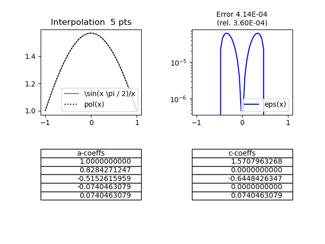
Polynomial approximation of \(sin(\frac{\pi}{2} x)/x\) computed on equally spaced points over the range \([-1,1]\). Top left: function and its approximation; Top right: absolute error; Bottom left: coefficients in the divided differences polynomial (basis: cumulated \(x - x_i\) products; Bottom right: approximation polynomial coefficients, in the monomial basis.
Calculating an interpolation polynomial using Newton's method of divided differences over an equally spaced points range of the target function values yields coefficients that are close to Hastings's approximation, but again not exactly equal.
3.4 Chebyshev nodes and polynomials
The Runge phenomenon, we alluded to before, is a problem of oscillation at the edges of an interval that occurs when using polynomial interpolation with polynomials of high degree over a reference of equispaced interpolation points. The polynomials produced by the Newton method over equally spaced points diverge away from \(f\) typically in an oscillating pattern that is amplified near the ends of the interpolation points.
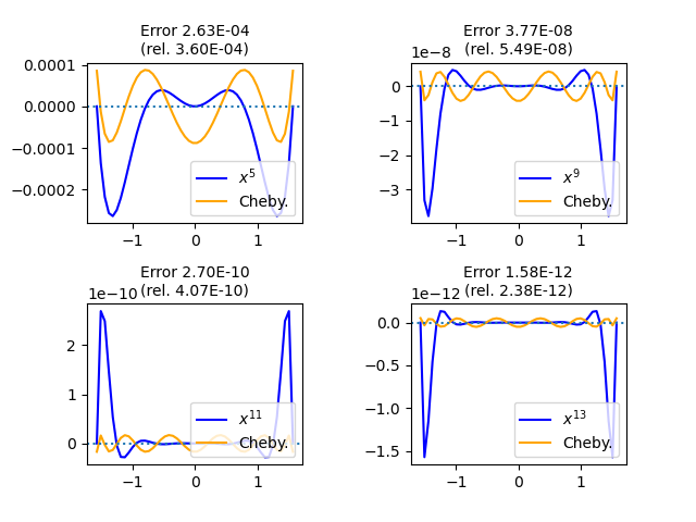
For instance the following graph compares the absolute error of the Newton polynomial approximations of \(\sin (x) / x\) over \([-\pi / 2, \pi / 2]\) for degrees 5, 9, 11, and 13 respectively:
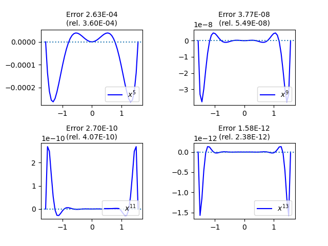
Runge Phenomenon for the function \( \sin (x) / x \). Paradoxically enough, the oscillations near the end points of the range quickly dwarf the ones closer to the center when the degree of the polynomial approximation increases.
In order to overcome this obstacle, we need to look into other references points for the calculation of the interpolant. Let us introduce the Chebyshev polynomials, named after Пафну́тий Льво́вич Чебышёв (1821-1894), a simple definition of which (by recurrence) is:
\begin{equation} T_0(x) = 1, \: T_1(x) = x, \: T_n(x) = 2 x T_{n-1}(x) - T_{n-2}(x), \: n \geq 2 \end{equation}This family of orthogonal polynomials has many properties of importance in varied areas of calculus. The results we are interested in for this investigation of the Moon Polynomiala are mainly:
- \(T_{n+1}\) has \(n+1\) distinct roots in \([-1, 1]\), called the Chebyshev nodes (of the first kind): \(x_k = \cos \frac{2 k + 1}{2 n + 2} \pi, \: k=0, 1, ... , n\)
- \(T_{n}\) has \(n+1\) distinct local extrema in \([-1, 1]\), called the Chebyshev nodes (of the second kind): \(t_k = \cos \frac{k}{n} \pi, \: k=0, 1, ... , n\)
- The minimax approximation of the zero function over \([-1,1]\) by a monic polynomial of degree \(n\) with real coefficients is \(\frac{ T_n(x) }{ 2^{ n - 1 } }\)
This last property, in particular, is used to prove that \(\max_{x \in [-1,1]} |(x - x_0) ... (x - x_n) |\) is minimal if and only if \((x - x_0) ... (x - x_n) = \frac{T_{n + 1}(x)}{2^n}\), i.e. if the \(x_k\) are the Chebyshev nodes of the first kind. So that if we seek better convergence of the minimax polynomial approximation we should most certainly use the Chebyshev nodes (of the first kind) as starting reference points.
Now, when we use the Chebyshev nodes instead of the equally spaced points to approximate the above \(\sin (x) / x\) function, the Runge phenomenon is subdued.
Subdued Runge Phenomenon for the function \( \sin (x) / x \), when using Chebyshev nodes of the first kind as reference points. End points oscillations have disappeared and almost equal oscillations are observed uniformally over the whole interval.
So let us start from the Chebyshev nodes to approximate the original \(\sin(\frac{\pi}{2} x)/x\) over the range \([-1,1]\) as used in the Apollo 11 source code:

Minimax approximation of the \(\sin(\frac{\pi}{2} x)/x\), using the Chebyshev nodes.
We are now getting much closer to the formula given by Hastings. Note first that the maximum relative error of the range is here \(0.0001342\); comparison with the Hastings polynomial approximation error looks like:

Comparing relative errors of approximation, i.e. \(\frac{p(x)-F(x)}{F(x)}\), for (i) the Hastings polynomial (blue line) and (ii) the Numpy-based Chebyshev nodes interpolant -- without refining iterations -- over the \([0,\pi/2]\) range (as both are symmetric). The maximum absolute difference in relative errors is 2.64 e-5, near \(x=1\) i.e. the \(x=\pi/2\) upper bound of the interval.
The Hastings polynomial provides a lower relative error near the extremities of the range compared to the simple interpolant constructed from the Chebyshev nodes references, without iterating the Remez algorithm (see later). The latter polynomial is a better approximation however on the subrange \([0.39783979 , 0.92739274]\).
3.5 Lagrange interpolation and the barycentric formula
We have so far applied theoretical results from the 19th century mathematical work alluded to in the introduction to our investigation of the Moon Polynomial. Taking stock the previous explorations, we express it into a comprehensive formulation, keeping in mind the sources of errors mentioned above.
Considering a basis \({\phi_j, j=0, ... n}\) of \(\mathcal{P}_n\), the interpolant \(p\) is most generally written as:
\begin{equation} p(x) = \sum_{j=0}^n c_j \phi_j(x) \end{equation}so that, given a trial reference \(x_i, \:y_i=f(x_i) \: i=0,1,...n\), the interpolation problem becomes, in matrix form:
\begin{equation} \label{eqn:matrix} \begin{pmatrix} \phi_0 (x_0) & \phi_1 (x_0) & ... & \phi_n (x_0) \\ \phi_0 (x_1) & \phi_1 (x_1) & ... & \phi_n (x_1) \\ \vdots & \vdots & & \vdots \\ \phi_0 (x_n) & \phi_1 (x_n) & ... & \phi_n (x_n) \end{pmatrix} \begin{pmatrix} c_0 \\ c_1 \\ \vdots \\ c_n \end{pmatrix} = \begin{pmatrix} y_0 \\ y_1 \\ \vdots \\ y_n \end{pmatrix} \end{equation}The choice of basis obviously appears crucial in the numerical solution to equation \ref{eqn:matrix}. The monomial basis \(\phi_j (x) = x^j\), as in the Taylor series for example, is usually a terrible choice Pachéon2009. On the other hand, the Chebyshev family of polynomials \(\phi_i (x) = T_i (x)\) is a a more sensible choice.
Experiments in the previous sections, with the exception of the truncated Taylor series, all used a Lagrange basis instead, named after Joseph-Louis Lagrange (born Giuseppe Luigi Lagrangia 1736-1813), where:
\begin{equation} \label{eqn:lagrange} \phi_j (x) = \mathcal{l}_j (x) = \frac{\prod_{k = 0, k \neq j}^n (x - x_k)}{\prod_{k = 0, k \neq j}^n (x_j - x_k)} \end{equation}
Notice that a Lagrange basis, in contrast to monomial and Chebyshev bases, is not prescribed beforehand but depends on data, i.e. on the trial reference and that \(l_j(x_i) = 1\) if \(i=j\) and \(0\) otherwise for \(i,j = 0, ... , n\). Our NumPy double precision experiments have further shown that a reference distribution for which the Lagrange interpolation is well-conditioned is indeed the Chebyshev nodes distribution (compared e.g. to the equally spaced reference).
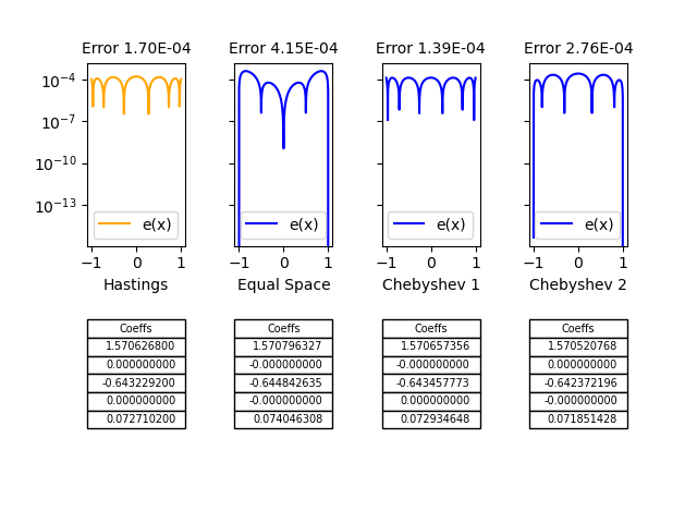
Lagrange interpolation on equally spaced references, Chebyshev nodes of the first kind and Chebyshev nodes of the second kind, compared to the Hastings polynomial approximation of 1955 used in the Apollo 11 code.
The previous approximation polynomials are recapitulated in the figure, where the Lagrange interpolation on Chebyshev nodes of the first kind appear closest, but not exactly identical, to the polynomial given by Hastings which was used in the extra-brief code for Apollo 11.
Nonetheless, among the shortcomings of the Lagrange interpolation sometimes claimed are the following:
- Each evaluation of \(p(x)\) requires \(O(n^2)\) additions and multiplications.
- Adding a newdata pair \((x_n+1, f_n+1)\) requires a new computation from scratch.
- The computation is numerically unstable with floating point mathematica libraries.
From the latter it is commonly concluded that the Lagrange form of \(p\) is mainly a theoretical tool for proving theorems. For numerical computations, it is generally recommended that one should instead use Newton's formula, which requires only \(O(n)\) floating point operations for each evaluation of \(p\) once some numbers, which are independent of the evaluation point \(x\), have been computed Trefethen2002.
The Lagrange formulation can be rewritten, however, in a way that it too can be evaluated and updated in \(O(n)\) operations: this is the barycentric formula. Indeed, the numerator of the expression \ref{eqn:lagrange} is simply \(\mathcal{l} (x) = (x - x_0) ... (x - x_n)\) divided by \((x - x_j)\). So by defining barycentric weights as \(w_j = \frac{1}{\prod_{k \neq j} (x_j - x_k)}\), then \(\mathcal{l}_j (x) = \mathcal{l} (x) \frac{w_j}{(x - x_j)}\) and finally:
\begin{equation} p(x) = \mathcal{l} (x) \sum_{j=0}^n \frac{w_j}{(x - x_j)} y_j \end{equation}Considering the Lagrange interpolation of the constant \(1\), we then get \(1 = \mathcal{l} (x) \sum_{j=0}^n \frac{w_j}{(x - x_j)}\), which used jointly with the previous expression finally yields the barycentric formula:
\begin{equation} p(x) = \frac{\sum_{j=0}^n \frac{w_j}{(x - x_j)} y_j}{\sum_{j=0}^n \frac{w_j}{(x - x_j)}} \end{equation}which is commonly used to compute the Lagrange interpolations because of its interesting properties. For instance, the weights \(w_j\) appear in the denominator exactly as in the numerator, except without the data factors \(y_j\). This means that any common factor in all the weights may be cancelled without affecting the value of \(p\).
In addition, for several node distributions the \(w_j\) have simple analytic definitions, which also speeds up the preparatory calculations. For equidistant references, for instance, \(w_j = (-1)^j \binom{n}{j}\). Note that if \(n\) is large, the weights for equispaced barycentric interpolation vary by exponentially large factors, of order approximately \(2^n\), leading to the Runge phenomenon. This distribution is ill-conditioned for the Lagrange interpolation. For the much better conditioned Chebyshev nodes, \(w_j = (-1)^j \sin \frac{(2 j + 1)\pi }{ 2 n + 2}\) which do not show the large variations found in the equally spaced reference distribution.
Other related node distributions can also be used in connection with other orthoginal polynomial families. For instance Legendre polynomials, named after Adrien-Marie Legendre (1752-1833), which are, like the Chebyshev polynomials, instances of the more general class of Jacobi polynomials, named after Carl Gustav Jacob Jacobi (1804-1851), provide a node distribution of the zeros of the degree 5 polynomial which can also be used as a trial reference, away from the Runge phenomenon.
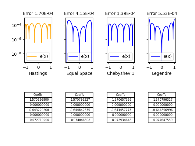
Lagrange interpolation on equally spaced references, Chebyshev nodes of the first kind and Legendre nodes, compared to the Hastings polynomial approximation of 1955 used in the Apollo 11 code.
Note that although the absolute error with the Legendre nodes is higher than with the Chebyshev nodes (of the first kind) but otherwise comparable, the median relative error \(5.668837 \: 10^{-5}\) is much lower than the Chebysev's \(9.659954 \: 10^{-5}\).
3.6 Remez algorithms
Can we get closer to the minimax solution to the continuous function approximation problem? Any continuous function on the interval \([a,b]\) is approximable by algebraic polynomials (a result due to Weierstrass). The map from such a function to its unique best approximation of degree \(n\) is non linear, so in 1934 Евгений Яковлевич Ремез (Evgeny Yakovlevich Remez, 1895-1975) following up on works by Félix Édouard Justin Émile Borel (1871-1956) and Charles-Jean Étienne Gustave Nicolas, baron de la Vallée Poussin (1866-1962) suggested a couple of iterative algorithms which under a broad range of assumptions converge on the minimax solution to the approximation problem Remez1934:2,Remez1934:1.
A first result is useful here: The equioscillation theorem attributed to Chebyshev, also proved by Borel, states that a polynomial \(p \in \mathcal{P}_n\) is the best approximation to \(f\) if and only if there exists a set of \(n+2\) distinct points \(x_i, i=0, ... , n+1\) such that \(f(x_i) - p(x_i) = s (-1)^i \| f - p^* \|\), and \(s = 1\) or \(s =-1\) is fixed. The unicity has been generally proven for polynomials under broader conditions by Alfréd Haar (1885-1933).
The second theorem used by Remez is due to de la Vallée Poussin and states a useful inequality: let \(p \in \mathcal{P}_n\) be any polynomial now such that the sign of the error alternates \(sign( f(z_i) - p(z_i) ) = s (-1)^i\) on a set of \(n+2\) points, \(z_i, i = 0, ... , n+1\), for any other \(q \in \mathcal{P}_n\), \(\min_i | f(z_i) - p(z_i) | \leq \max_i | f(z_i) - q(z_i) |\) and in particular \(\min_i | f(z_i) - p(z_i) | \leq \| f - p^* \| \leq \| f - p \|\).
Remez algorithms iteratively compute sequences of references and polynomials such thar the error equioscillates at each step and \(\frac{\| f - p \|}{\min_i | f(z_i) - p(z_i) |} \rightarrow 1\). Each iteration relies on first solving the system \(n+2\) equations \(f(z_i) - p(z_i) = s (-1)^i \varepsilon\) to obtain the coefficients of polynomial \(p\) and the error \(\varepsilon\), and secondly locate the extrema of the new approximation error function, and use these as new reference points for the next iteration.
Experiments with double precision in NumPy did not produce significant improvement over the Lagrange interpolation on Chebyshev nodes (of the first kind) studied earlier. Indeed as shown above the approximation is already very close to the function used by Hastings. For better accuracy we ran the Remez algorithms as implemented in Sollya, both a tool environment and a library for safe floating-point code development ChevillardJoldesLauter2010. The coefficients of the best approximation polynomial to $sin ( \frac{\pi}{2} x ) / x
$ from Sollya are:
| Coefficient | Monomial |
|---|---|
| 1.57065972900121206782476772668946411106733878714064 | \(x^0\) |
| 6.3492906909712336205872528382574323066525019450686 e-13 | \(x\) |
| -0.64347673917200615933412286446370386788140592486393 | \(x^2\) |
| -1.98174331531856942836713657192082059845357482792894 e-12 | \(x^3\) |
| 0.072953607963105953292564355389989278883511381946124 | \(x^4\) |
The Remez algorithm produces also a polynomial which is close to the simple Lagrange interpolation in the previous section conforting our candidate compared to the one in Hastings5.
4 Conclusions
Historically then it seems that the Moon Polynomial that served during the Apollo mission was a remarkably efficient assembly language implementation of the approximation published by Hastings in 1955. Reimplementing different construction of double-precision interpolants and best approximations produces various polynomials of the same degree with coefficients close, but not exactly similar to Hastings'. Meanwhile a too long procrastinated delve into Milton Abramowitz and Irene Stegun's comprehensive Handbook of Mathematical Functions with Formulas, Graphs, and Mathematical Tables (1964) AbramowitzStegun1964 tells us that Ruth Zucker in her chapter about Circular Functions refers to two works for the sine function:
- The now famous November 1954 Rand Corp. report by Cecil Hastings, Jr., assisted by Jeanne T. Hayward and James P. Wong, Jr.: Approximations for Digital Computers, on p. 138 (Sheet 14 of Part 2) Hastings:1955; but also
- An August 1955 Los Alamos Laboratory (LA 1943) by Bengt Carlson and Max Goldstein: Rational Approximations of Functions, on p. 34-38 Carlson:1955, with thanks to Chester S. Kazek, Jr. and Josephine Powers.
Hastings himself cites Approximations With Least Maximum Error by R. G. Selfridge (1953) Selfridge1953 and A Short Method for Evaluating Determinants and Solving Systems of Linear Equations with Real or Complex Coefficients by Prescott Durand Crout Crout1941 for further details on the (part manual, part computerized) algorithm to construct the polynomial.
4.1 The sine function at the Los Alamos Lab
Several tables for \(sin(x)/x\) are provided in the Los Alamos Lab Technical Report for "optimum rational approximators". The authors, however, warn:
The method,to be described below, for obtaining optimum approximators is essentially an empirical one which proceeds toward the final solution in aniterative manner. It has proven to be rapidly convergent in the many applications made to date, and it is, therefore, hoped that the method may eventually be put on a firm mathematical basis.
The firm basis was solidly established when accurate interpolations were once again required in filter design for signal processing. The Parks–McClellan algorithm, published by James McClellan and Thomas Parks in 1972, is an iterative algorithm for finding the optimal Chebyshev finite impulse response (FIR) filter. The Parks–McClellan algorithm is used to design and implement efficient and optimal FIR filters. This renewed interest in polynomial approximation prompted new lines of investigations and the revisiting of the works of pioneer mathematicians at the turn of the 20th century.
On page 34 the following tables are provided for the expansion on \([0, \pi/2]\):
\begin{equation} \frac{sin(x)}{x} = a_0 + a_1x^2 + a_2x^4 + ... + a_nx^{2n} \end{equation}| n=2 | n=3 | n=4 | n=5 | |
|---|---|---|---|---|
| rel | .00017 | .0000013 | .0000000069 | .0000000002 |
| \(a_0\) | 1.00000 00000 | 1.00000 00000 | 1.00000 00000 | 1.00000 00000 |
| \(a_1\) | -.16605 37570 | -.16665 76051 | -.16666 65880 | -.16666 66664 |
| \(a_2\) | .00761 17733 | .00831 28622 | .00833 30455 | .00833 33315 |
| \(a_3\) | -.00018 49551 | -.00019 80800 | -.00019 84090 | |
| \(a_4\) | .00000 26021 | .00000 27526 | ||
| \(a_5\) | -.00000 00239 |
Selecting the \(n=2\) column for comparing interpolants and scaling back to the Hastings target function:
| Hastings | Los Alamos | Lagrange Int. | Remez/Sollya |
|---|---|---|---|
| 1.5706268 | 1.5707963 | 1.5706574 | 1.5706597 |
| -0.6432292 | -0.6435886 | -0.6434578 | -0.6434767 |
| 0.0727102 | 0.0727923 | 0.0729346 | 0.0729536 |
Note that the Hastings polynomial has clearly outlier coefficients when compared to the other traditional constructions:
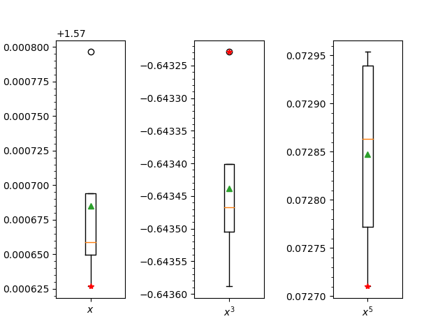
Box plots for the three coefficients of monomials in the four contructions: Hastings, Los Alamos, Lagrange interpolation (on Chebyshev nodes) and Sollya Remez algorithm implementation. Median values are orange, means in green and red are the Hastings coefficients.
The medians and means are in the following table:
| Median | Mean |
|---|---|
| 1.5706585 | 1.5706851 |
| -0.6434673 | -0.6434381 |
| 0.0728635 | 0.0728477 |
4.2 Modern sines of the times
4.2.1 Netlib/fdlibm
Of course polynomial interpolants of the sine functions served many endeavours besides putting Man on the Moon. Consider for instance Netlib, a repository of software for scientific computing maintained by AT&T, Bell Laboratories, the University of Tennessee and Oak Ridge National Laboratory, started in the late eighties Dongarra87. In this trove of mathematical software the implementation of the sine function if found in the fdlibm library.
			*********************************
			* Announcing FDLIBM Version 5.3 *
			*********************************
			============================================================
                        FDLIBM
			============================================================
			developed at Sun Microsystems, Inc.

			FDLIBM is intended to provide a reasonably portable (see
			assumptions below), reference quality (below one ulp for
			major functions like sin,cos,exp,log) math library
			(libm.a).  For a copy of FDLIBM, please see
			http://www.netlib.org/fdlibm/
			or
			http://www.validlab.com/software/
The sine function is indeed implemented through the evaluation of a polynomial interpolant with the following coefficients from the 1993-dated version of the source code:
| Coefficient (decimal) | (hex) | (hex) |
|---|---|---|
| S1 = -1.66666666666666324348e-01 | /* 0xBFC55555 | 0x55555549 */ |
| S2 = 8.33333333332248946124e-03 | /* 0x3F811111 | 0x1110F8A6 */ |
| S3 = -1.98412698298579493134e-04 | /* 0xBF2A01A0 | 0x19C161D5 */ |
| S4 = 2.75573137070700676789e-06 | /* 0x3EC71DE3 | 0x57B1FE7D */ |
| S5 = -2.50507602534068634195e-08 | /* 0xBE5AE5E6 | 0x8A2B9CEB */ |
| S6 = 1.58969099521155010221e-10 | /* 0x3DE5D93A | 0x5ACFD57C */ |
which are one step further the monomial exponent series from the Los Alamos \(n=5\) reference column (agreeing to the 8th decimal).
4.2.2 GSL and GLIBC
Other modern sines are found in the GNU Scientific Library (GSL), a numerical library for C and C++ programmers. It is free software under the GNU General Public License. The library provides a wide range of mathematical routines such as random number generators, special functions and least-squares fitting. There are over 1000 functions in total with an extensive test suite. In gsl1.0 dated 2001, the sine function used different approximations according to the value of its argument \(x\). One of the interpolants is represented as its decomposition on Chebyshev polynomials (to order 11):
/* specfunc/trig.c
			 *
			 * Copyright (C) 1996, 1997, 1998, 1999, 2000 Gerard Jungman
			 *
			 * This program is free software; you can redistribute it and/or modify
			 * it under the terms of the GNU General Public License as published by
			 * the Free Software Foundation; either version 3 of the License, or (at
			 * your option) any later version.
			 *
			*/

			/* Chebyshev expansion for f(t) = g((t+1)Pi/8), -1<t<1
			 * g(x) = (sin(x)/x - 1)/(x*x)
			 */
			static double sin_data[12] = {
			-0.3295190160663511504173,
			0.0025374284671667991990,
			0.0006261928782647355874,
			-4.6495547521854042157541e-06,
			-5.6917531549379706526677e-07,
			3.7283335140973803627866e-09,
			3.0267376484747473727186e-10,
			-1.7400875016436622322022e-12,
			-1.0554678305790849834462e-13,
			5.3701981409132410797062e-16,
			2.5984137983099020336115e-17,
			-1.1821555255364833468288e-19
			};
which has not changed up to the current version dated March 2019.
For values close to \(0\), the Taylor expansion is used. Away from this boundary the Chebyshev interpolant above is used and the absolute error if of the order of \(10^{-13}\) over the \([-1 + \varepsilon , 1]\) interval.
The 11th order Chebyshev approximation used for the sine function in the GSL. Away from 0 the absolute error is within 1e-13
In glibc, the GNU C Library project that provides the core libraries for the GNU system and GNU/Linux systems, as well as many other systems that use Linux as the kernel, the libraries provide critical APIs including ISO C11, POSIX.1-2008, BSD, OS-specific APIs and more. The double 64 bits implementation of the sine function (in s_sin.c) reads:
/*
			 * IBM Accurate Mathematical Library
			 * written by International Business Machines Corp.
			 * Copyright (C) 2001-2020 Free Software Foundation, Inc.
			 *
			*/
			/****************************************************************************/
			/*                                                                          */
			/* MODULE_NAME:usncs.c                                                      */
			/*                                                                          */
			/* FUNCTIONS: usin                                                          */
			/*            ucos                                                          */
			/* FILES NEEDED: dla.h endian.h mpa.h mydefs.h  usncs.h                     */
			/*               branred.c sincos.tbl                                       */
			/*                                                                          */
			/* An ultimate sin and cos routine. Given an IEEE double machine number x   */
			/* it computes sin(x) or cos(x) with ~0.55 ULP.                             */
			/* Assumption: Machine arithmetic operations are performed in               */
			/* round to nearest mode of IEEE 754 standard.                              */
			/*                                                                          */
			/****************************************************************************/
			/* Helper macros to compute sin of the input values.  */
			#define POLYNOMIAL2(xx) ((((s5 * (xx) + s4) * (xx) + s3) * (xx) + s2) * (xx))

			#define POLYNOMIAL(xx) (POLYNOMIAL2 (xx) + s1)

			/* The computed polynomial is a variation of the Taylor series expansion for
			   sin(a):

			   a - a^3/3! + a^5/5! - a^7/7! + a^9/9! + (1 - a^2) * da / 2

			   The constants s1, s2, s3, etc. are pre-computed values of 1/3!, 1/5! and so
			   on.  The result is returned to LHS.  */
			static const double
			sn3 = -1.66666666666664880952546298448555E-01,
			sn5 = 8.33333214285722277379541354343671E-03,
which shows the use of the truncated Taylor series expansion. In the header file usncs.h, a larger truncation of the series is provided:
#ifndef USNCS_H
			#define USNCS_H

			static const double s1 = -0x1.5555555555555p-3;   /* -0.16666666666666666     */
			static const double s2 = 0x1.1111111110ECEp-7;    /*  0.0083333333333323288   */
			static const double s3 = -0x1.A01A019DB08B8p-13;  /* -0.00019841269834414642  */
			static const double s4 = 0x1.71DE27B9A7ED9p-19;   /*  2.755729806860771e-06   */
			static const double s5 = -0x1.ADDFFC2FCDF59p-26;  /* -2.5022014848318398e-08  */
which is close but slightly different from the interpolant used above in fdlibm.
4.2.3 BASIC for microcomputers
An older but classical implementation is found in the sine function in Microsoft's 6502 BASIC.
		      ;SINE FUNCTION.
		      ;USE IDENTITIES TO GET FAC IN QUADRANTS I OR IV.
		      ;THE FAC IS DIVIDED BY 2*PI AND THE INTEGER PART IS IGNORED
		      ;BECAUSE SIN(X+2*PI)=SIN(X). THEN THE ARGUMENT CAN BE COMPARED
		      ;WITH PI/2 BY COMPARING THE RESULT OF THE DIVISION
		      ;WITH PI/2/(2*PI)=1/4.
		      ;IDENTITIES ARE THEN USED TO GET THE RESULT IN QUADRANTS
		      ;I OR IV. AN APPROXIMATION POLYNOMIAL IS THEN USED TO
		      ;COMPUTE SIN(X).
		      SIN:	JSR	MOVAF
		      LDWDI	TWOPI		;GET PNTR TO DIVISOR.
		      LDX	ARGSGN		;GET SIGN OF RESULT.
		      JSR	FDIVF
		      JSR	MOVAF		;GET RESULT INTO ARG.
		      JSR	INT		;INTEGERIZE FAC.
		      CLR	ARISGN		;ALWAYS HAVE THE SAME SIGN.
		      JSR	FSUBT		;KEEP ONLY THE FRACTIONAL PART.
		      LDWDI	FR4		;GET PNTR TO 1/4.
		      JSR	FSUB		;COMPUTE 1/4-FAC.
		      LDA	FACSGN		;SAVE SIGN FOR LATER.
		      PHA
		      BPL	SIN1		;FIRST QUADRANT.
		      JSR	FADDH		;ADD 1/2 TO FAC.
		      LDA	FACSGN		;SIGN IS NEGATIVE?
		      BMI	SIN2
		      COM	TANSGN		;QUADRANTS II AND III COME HERE.
		      SIN1:	JSR	NEGOP		;IF POSITIVE, NEGATE IT.
		      SIN2:	LDWDI	FR4		;POINTER TO 1/4.
		      JSR	FADD		;ADD IT IN.
		      PLA			;GET ORIGINAL QUADRANT.
		      BPL	SIN3
		      JSR	NEGOP		;IF NEGATIVE, NEGATE RESULT.
		      SIN3:	LDWDI	SINCON
		      GPOLYX: JMP	POLYX		;DO APPROXIMATION POLYNOMIAL.


		      PAGE
		      SUBTTL	POLYNOMIAL EVALUATOR AND THE RANDOM NUMBER GENERATOR.
		      ;EVALUATE P(X^2)*X
		      ;POINTER TO DEGREE IS IN [Y,A].
		      ;THE CONSTANTS FOLLOW THE DEGREE.
		      ;FOR X=FAC, COMPUTE:
		      ; C0*X+C1*X^3+C2*X^5+C3*X^7+...+C(N)*X^(2*N+1)
		      POLYX:	STWD	POLYPT		;RETAIN POLYNOMIAL POINTER FOR LATER.
		      JSR	MOV1F		;SAVE FAC IN FACTMP.
		      LDAI	TEMPF1
		      JSR	FMULT		;COMPUTE X^2.
		      JSR	POLY1		;COMPUTE P(X^2).
		      LDWDI	TEMPF1
		      JMP	FMULT		;MULTIPLY BY FAC AGAIN.

		      ;POLYNOMIAL EVALUATOR.
		      ;POINTER TO DEGREE IS IN [Y,A].
		      ;COMPUTE:
		      ; C0+C1*X+C2*X^2+C3*X^3+C4*X^4+...+C(N-1)*X^(N-1)+C(N)*X^N.
		      POLY:	STWD	POLYPT
		      POLY1:	JSR	MOV2F		;SAVE FAC.
		      LDADY	POLYPT
		      STA	DEGREE
		      LDY	POLYPT
		      INY
		      TYA
		      BNE	POLY3
		      INC	POLYPT+1
		      POLY3:	STA	POLYPT
		      LDY	POLYPT+1
		      POLY2:	JSR	FMULT
		      LDWD	POLYPT		;GET CURRENT POINTER.
		      CLC
		      ADCI	4+ADDPRC
		      BCC	POLY4
		      INY
		      POLY4:	STWD	POLYPT
		      JSR	FADD		;ADD IN CONSTANT.
		      LDWDI	TEMPF2		;MULTIPLY THE ORIGINAL FAC.
		      DEC	DEGREE		;DONE?
		      BNE	POLY2
		      RANDRT: RTS			;YES.

		      SINCON: 5		;DEGREE-1.
		      204	; -14.381383816
		      346
		      032
		      055
		      033
		      206	; 42.07777095
		      050
		      007
		      373
		      370
		      207	; -76.704133676
		      231
		      150
		      211
		      001
		      207	; 81.605223690
		      043
		      065
		      337
		      341
		      206	; -41.34170209
		      245
		      135
		      347
		      050
		      203	; 6.2831853070
		      111
		      017
		      332
		      242
		      .;E063 05                        6 coefficients for SIN()
		      .;E064 84 E6 1A 2D 1B            -((2*PI)**11)/11! = -14.3813907
		      .;E069 86 28 07 FB F8             ((2*PI)**9)/9!   =  42.0077971
		      .;E06E 87 99 68 89 01            -((2*PI)**7)/7!   = -76.7041703
		      .;E073 87 23 35 DF E1             ((2*PI)**5)/5!   =  81.6052237
		      .;E078 86 A5 5D E7 28            -((2*PI)**3)/3!   = -41.3147021
		      .;E07D 83 49 0F DA A2               2*PI           =  6.28318531
A look at the coefficient of the approximation polynomial reveals that it is a truncated Taylor series (up to \(x^{11}\)) quite comparable to the series used in s_sin.c from glibc. Note that including the code for the polynomial evaluation and the conditioning of the argument, the source far exceeds the concise \(35\) lines of the AGC. On the other hand, there is no native instruction for floating point multiplication. It is implemented in the FMULT procedure which adds another hundred or so lines of assembly code.
By comparison the NASCOM ROM BASIC ver. 4.7, by Microsoft in 1978, shows the following coefficients for the sine approximation polynomial:
		      SINTAB: .BYTE   5                       ; Table used by SIN
		      .BYTE   0BAH,0D7H,01EH,086H     ; 39.711
		      .BYTE   064H,026H,099H,087H     ;-76.575
		      .BYTE   058H,034H,023H,087H     ; 81.602
		      .BYTE   0E0H,05DH,0A5H,086H     ;-41.342
		      .BYTE   0DAH,00FH,049H,083H     ;  6.2832
where the truncation is at \(x^9\) rather than \(x^{11}\) for the 6502.
In the Z80 BBC BASIC,
		      ;
		      ;Z80 FLOATING POINT PACKAGE
		      ;(C) COPYRIGHT  R.T.RUSSELL  1986
		      ;VERSION 0.0, 26-10-1986
		      ;VERSION 0.1, 14-12-1988 (BUG FIX)

		      ;;SIN - Sine function
		      ;Result is floating-point numeric.
		      ;
		      SIN:    CALL    SFLOAT
		      SIN0:   PUSH    HL              ;H7=SIGN
		      CALL    SCALE
		      POP     AF
		      RLCA
		      RLCA
		      RLCA
		      AND     4
		      XOR     E
		      SIN1:   PUSH    AF              ;OCTANT
		      RES     7,H
		      RRA
		      CALL    PIBY4
		      CALL    C,RSUB          ;X=(PI/4)-X
		      POP     AF
		      PUSH    AF
		      AND     3
		      JP      PO,SIN2         ;USE COSINE APPROX.
		      CALL    PUSH5           ;SAVE X
		      CALL    SQUARE          ;PUSH X*X
		      CALL    POLY
		      DEFW    0A8B7H          ;a(8)
		      DEFW    3611H
		      DEFB    6DH
		      DEFW    0DE26H          ;a(6)
		      DEFW    0D005H
		      DEFB    73H
		      DEFW    80C0H           ;a(4)
		      DEFW    888H
		      DEFB    79H
		      DEFW    0AA9DH          ;a(2)
		      DEFW    0AAAAH
		      DEFB    7DH
		      DEFW    0               ;a(0)
		      DEFW    0
		      DEFB    80H
		      CALL    POP5
		      CALL    POP5
		      CALL    FMUL
		      JP      SIN3
the approximation is a degree \(4\) polynomial in \(x^2\). The coefficients are declared following the DEFW as 32 bit sign-magnitude normalized mantissa followed by an (DEFB) 8 bit excess-128 signed exponent. Converted to floating point decimals, these resolve to the double of the following (absolute) values:
| Coefficients |
|---|
| 0.16666666587116197 |
| 0.00833321735262870 |
| 0.00020314738375600 |
| 0.00000264008694502 |
which are close enough to the \(n=4\) Los Alamos Lab polynomial's.
Hence, in spite of the few known methods of interpolation and numerical approximation dating back to the 50s, many different polynomials were used in the microcomputer BASIC implementations during the late 70s and the 80s with varied levels of accuracy. But none of it as concise as the Moon polynomial!
4.2.4 NumPy
And so, in NumPy, it should now come at no surprise to the patient reader that the circular functions are also implemented as polynomial approximations! So that speculations that the experiments of the previous sections simply ended up in comparing an implementation of one candidate polynomial to the implementation of another one are definitely legitimate.
One of the NumPy implementation of the sine function is found in the fft module, namely the _pocketfft.c file where:
/*
			 * This file is part of pocketfft.
			 * Licensed under a 3-clause BSD style license - see LICENSE.md
			 */

			/*
			 *  Main implementation file.
			 *
			 *  Copyright (C) 2004-2018 Max-Planck-Society
			 *  \author Martin Reinecke
			 */

			// CAUTION: this function only works for arguments in the range [-0.25; 0.25]!
			static void my_sincosm1pi (double a, double *restrict res)
			{
			double s = a * a;
			/* Approximate cos(pi*x)-1 for x in [-0.25,0.25] */
			double r =     -1.0369917389758117e-4;
			r = fma (r, s,  1.9294935641298806e-3);
			r = fma (r, s, -2.5806887942825395e-2);
			r = fma (r, s,  2.3533063028328211e-1);
			r = fma (r, s, -1.3352627688538006e+0);
			r = fma (r, s,  4.0587121264167623e+0);
			r = fma (r, s, -4.9348022005446790e+0);
			double c = r*s;
			/* Approximate sin(pi*x) for x in [-0.25,0.25] */
			r =             4.6151442520157035e-4;
			r = fma (r, s, -7.3700183130883555e-3);
			r = fma (r, s,  8.2145868949323936e-2);
			r = fma (r, s, -5.9926452893214921e-1);
			r = fma (r, s,  2.5501640398732688e+0);
			r = fma (r, s, -5.1677127800499516e+0);
			s = s * a;
			r = r * s;
			s = fma (a, 3.1415926535897931e+0, r);
			res[0] = c;
			res[1] = s;
			}
The author also refers to "Implementation of sinpi() and cospi() using standard C math library", a post on the Web site stackoverflow, which has further historical comments. The main observation here is that this C99 code relies heavily on the use of \(fma()\), which implements a fused multiply-add operation. On most modern hardware architectures, this is directly supported by a corresponding hardware instruction. Where this is not the case, the code may experience significant slow-down due to generally slow FMA emulation.
The code above compute the following polynomial \(P(x) = \pi*x + x*x*x*( x*x*(x*x*(x*x*(x*x*(x*x*4.6151442520157035e-4 + -7.3700183130883555e-3) + 8.2145868949323936e-2) -5.9926452893214921e-1) + 2.5501640398732688e+0) -5.1677127800499516e+0)\). Changing variables to match the Hastings function resolves it to \(P(t) = 5.633721010761356811523437500 E-8*t^{12} - 3.598641754437673583984375000 E-6*t^{10} + 0.0001604411502916483125000000000*t^8 - 0.004681754132282415703125000000*t^6 + 0.07969262624603965000000000000*t^4 - 0.6459640975062439500000000000*t^2+ 1.570796326794896619231321692\)
The coefficients up to the 12th-degree are compared to the degree 9 polynomial given by Hastings (sheet 16, p. 140 of Hastings:1955) in the following table:
| NumPy | Hastings |
|---|---|
| 1.57079632679 | 1.57079631847 |
| 0 | 0 |
| - 0.64596409751 | - 0.64596371106 |
| 0 | 0 |
| 0.07969262625 | 0.07968967928 |
| 0 | 0 |
| - 0.00468175413 | - 0.00467376557 |
| 0 | 0 |
| 0.00016044115 | 0.00015148419 |
| 0 | 0 |
| - 0.00000359864 | - |
| 0 | - |
| 0.00000005634 | - |
Note that Hastings's approximation is given for \([ - \pi / 2, \pi / 2 ]\) while the NumPy polynomial approximation is valid for \([ - \pi / 4, \pi / 4 ]\) as explicitly mentioned in the source code. Coefficients are identical up to the fifth decimal, but as usual the Hastings approximation aims at a minimal relative error while this \(P\) is geared towards minimizing absolute error.
In order to compare to the Los Alamos polynomials, we need to change variables again to target \(\sin(x) / x\), obtaining \(P(t) = 1.589413637225924385400714899 E-10*t^{13} - 2.505070584638451291215866027 E-8*t^{11} + 2.755731329901509726061486689 E-6*t^9 - 0.0001984126982840212156257908627*t^7 + 0.008333333333320011824754439271*t^5 - 0.1666666666666660722952030262*t^3 + 1.000000000000000000000000000*t\). The following table now compares these coefficients to the maximum degree (\(8\)) polynomial approximation given in the Los Alamos technical report (p. 35 of Carlson:1955) for the same range \([ - \pi / 4, \pi / 4 ]\):
| NumPy | Los Alamos | Los Alamos "Expansion" |
|---|---|---|
| 1 | 1 | 1 |
| 0 | 0 | 0 |
| - 0.1666666667 | - 0.1666666667 | - 0.1666666667 |
| 0 | 0 | 0 |
| 0.0083333333 | 0.0083333327 | 0.0083333333 |
| 0 | 0 | 0 |
| - 0.0001984127 | - 0.0001984036 | - 0.0001984127 |
| 0 | 0 | 0 |
| 0.0000027557 | 0.0000027274 | 0.0000027557 |
| 0 | 0 | 0 |
| - 0.0000000251 | - | - 0.0000000251 |
| 0 | - | 0 |
| 0.0000000002 | - | 0.0000000002 |
The last column, called "Expansion" in the Los Alamos technical report is simply the Taylor/McLaurin expansion of the target function. Note that its coefficients are exactly the ones of the NumPy approximation, while the report suggests a shorter approximation polynomial with (naturally) slightly different coefficients. So this NumPy implementation is yet another example of resorting to the Taylor expansion.
4.3 Ancient sines: brevity and arbitrary precision
The "modern sines", through their numerical approximation and the zoology of interpolant polynomials, provide appropriate compromise between brevity and accuracy according to the machine architecture and the objectives to be met. Interestingly enough, as sines numerical tables obviously predate the modern computer, some tables are found for instance in Ancient Greece literature, could the "ancient sines" of the Elder throw some additional light on the question?
Although it has been known for a long time that in the 16th century the Swiss clockmaker at the court of William IV, Landgrave of Hesse-Kassel, Jost Bürgi (1552-1632) found a new method for calculating sines, no information about the details has been available. In a letter of the Prince to astronomer Tycho Brahe (1546-1601) Bürgi was praised as a "second Archimedes", and in 1604, he entered the service of emperor Rudolf II in Prague. Here, he befriended the royal astronomer Johannes Kepler (1571-1630) and constructed a table of sines (Canon Sinuum), which was supposedly very accurate. It is clear from letters exchanged between Brahe, Kepler and other astronomers of the times that such accurate tables, like the comprehensive tables of precise astronomical observations, of which Brahe's Tabulae Rudolphinae were a superb example that drew admiration (and envy) all over the royal courts of Europe, were considered as (trade) secrets and protected as such, as patents are today.
In 2015, however, a manuscript written by Bürgi himself came to light in which he explains his algorithm. It is totally different from the traditional procedure which was used until the 17th century folkerts2015. While the standard method was rooted in Greek antiquity with Ptolemy's computation of chords and used in the Arabic-Islamic tradition and in the Western European Middle Ages for calculating chords as well as sines, Bürgi's way, he called KunstWeg was not. By only using additions and halving, his procedure is elementary and it converges quickly. (Bürgi does not explain why his method is correct, but folkerts2015 provides a modern proof for the correctness of the algorithm.)
Bürgi’s algorithm is deceptively simple. There is no bisection, no roots, only two basic operations: many additions, and a few divisions by 2. The computations can be done with integers, or with sexagesimal values, or in any other base FOLKERTS2016133. In order to compute the sines, Bürgi starts with an arbitrary list of values, which can be considered as first approximations of the sines, but need not be. The principles of iterative sine table calculation through the Kunstweg are as follows: cells in a column sum up the values of the two cells in the same and previous column. The final cell's value is divided by two, and the next iteration starts. Finally, the values of the last column get normalized. Rather accurate approximations of sines are obtained after only a few iterations. This scheme can be adapted to obtain any set of values \(\sin( k \pi / 2n )\), for \(0 \leq k \leq n\), but it is important to realize that this algorithm provides all the values, and cannot provide only one sine. All the sines are obtained in parallel, with relatively simple operations.
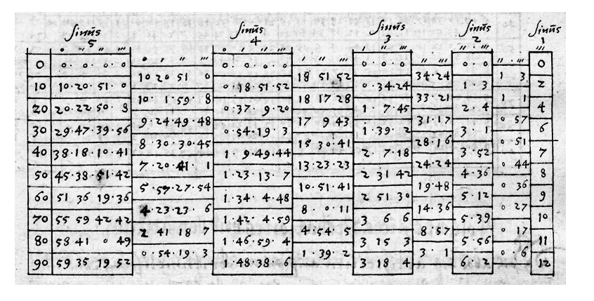
Figure 12: Bürgi's KunstWeg in Fundamentum Astronomiae, fol. 36R, and its decimal translation as provided by folkerts2015
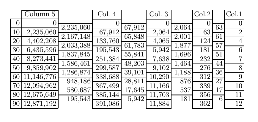
the sines are obtained by normalising the last column, on the left, dividing each cell by the last one \(12,871,192\), yielding \(\sin 10^{\circ}, \sin 20^{\circ} ... \sin 90^{\circ}\).
Because the sine table in Georg Joachim de Porris, also known as Rheticus (1514-1574) (an astronomer himself and a pupil of Nicolaus Copernicus) Opus Palatinum, which had been printed in 1596, contained many errors, Bürgi later computed another, even more detailed sine table for every two seconds of arc, thus containing 162,000 sine values! (A towering work of numerical computation.) This table has not survived. Bürgi took special care that his method of calculating sines did not become public in his time. Only since his Fundamentum Astronomiae has been found, do we know with certainty that he made use of tabular differences, reminiscent of the Newton method presented earlier.
And to quote folkerts2015, "Indeed, as we have seen, this process has unexpected stability properties leading to a quickly convergent sequence of vectors that approximate this eigenvector [in the modern proof] and hence the sine-values. The reason for its convergence is more subtle than just some geometric principle such as exhaustion, monotonicity, or Newton’s method, it rather relies on the equidistribution of a diffusion process over time –- an idea which was later formalized as the Perron-Frobenius theorem and studied in great detail in the theory of Markov chains. Thus, we must admit that Bürgi’s insight anticipates some aspects of ideas and developments that came to full light only at the beginning of the 20th century."
How ironic that the Moon Polynomial was unrelated to the inventive clockmaker KunstWeg, so much praised by the prime astronomers of the European 16th and 17th century!
Bibliography
- [Pachéon2009] Pachéon & Trefethen, Barycentric-Remez algorithms for best polynomial approximation in the chebfun system, BIT Numerical Mathematics, 49(4), 721 (2009). link. doi.
- [Remez1934:2] Eugene Remes, Sur le calcul effectif des polynomes d'approximation de Tchebichef., Comptes rendus hebdomadaires des séances de l'Académie des sciences. (1934).
- [Parks1972] Parks & McClellan, Chebyshev Approximation for Nonrecursive Digital Filters with Linear Phase, IEEE Transactions on Circuit Theory, 19(2), 189-194 (1972).
- [AGC2010] Frank O'Brien, The Apollo Guidance Computer, Praxis (2010).
- [Hastings:1955] Cecil Hastings, Approximations for Digital Computers, pub-PRINCETON (1955).
- [Johansson2015] Johansson, Efficient implementation of elementary functions in the medium-precision range, (2015).
- [Trefethen2002] Trefethen, Barycentric Lagrange Interpolation, SIAM Review, 46, (2002). doi.
- [Remez1934:1] Eugene Remes, Sur un procédé convergent d'approximations successives pour déterminer les polynomes d'approximation., Comptes rendus hebdomadaires des séances de l'Académie des sciences. (1934).
- [ChevillardJoldesLauter2010] ~Chevillard, Joldes & Lauter, Sollya: An Environment for the Development of Numerical Codes, Springer (2010).
- [AbramowitzStegun1964] Abramowitz & Stegun, Handbook of Mathematical Functions with Formulas, Graphs, and Mathematical Tables, Dover (1964).
- [Carlson:1955] Bengt Carlson & Max Goldstein, Rational Approximations of Functions, inst-LASL, (1955).
- [Selfridge1953] "Selfridge, Approximations with least maximum error., "Pacific J. Math.", 3(1), 247-255 (1953). link.
- [Crout1941] Crout, A short method for evaluating determinants and solving systems of linear equations with real or complex coefficients, Electrical Engineering, 60(12), 1235-1240 (1941).
- [Dongarra87] Jack Dongarra, Distribution of mathematical software via electronic mail, Communications of the ACM, 30, 403-407 (1987).
- [folkerts2015] Menso Folkerts, Dieter Launert & Andreas Thom, Jost Bürgi's Method for Calculating Sines, , (2015).
- [FOLKERTS2016133] "Menso Folkerts, Dieter Launert & Andreas Thom", Jost Bürgi's method for calculating sines, "Historia Mathematica", 43(2), 133 - 147 (2016). link. doi.
- [Lanczos:1938:TIE] "Lanczos", Trigonometric Interpolation of Empirical and Analytical Functions, "Journal of mathematics and physics Massachusetts Institute of Technology", 17(??), 123-199 (1938).
- [Golub1971] Golub & Smith, Algorithm 414: Chebyshev Approximation of Continuous Functions by a Chebyshev System of Functions, Commun. ACM, 14(11), 737–746 (1971). link. doi.
- [Stroethoff2014] Karel Stroethoff, Bhaskara’s approximation for the Sine, The Mathematical Enthusiast, 11(3), 485-494 (2014).
Footnotes:
It can also be found in the master repository of the Apollo 11 computer simulation project: http://www.ibiblio.org/apollo/.
By the Weierstrass approximation theorem, after Karl Theodor Wilhelm Weierstrass (1815-1897), for any set of \(n + 1\) values \(y_0, ..., y_n\) located at distinct points \(x_0, ... , x_n\), there exists a unique polynomial of degree \(n\), denoted by \(p_n\), which exactly passes through each of the \(n + 1\) points. This polynomial is called an interpolant. Likewise functions can be interpolated: \(p_n\) is the unique interpolant with degree \(n\) of a function \(f\) at points \(x_0, ... , x_n\) if \(P_n(x_i) = f(x_i)\) for all \(i = 0, ... , n\).
Hasting's book gives polynomial approximations of degrees 5, 7 and 9. The Los Alamos book gives polynomial approximations of degrees 5, 7, 9 and 11 on two intervals (\([0 , \pi/4]\) and \([0 , \pi/2]\)) but also continued products/fractions. The Indian mathematician Bhaskara I (c. 600-c. 680) gave the rational approximation \(sin(x) \approx \frac{16x(\pi - x)}{5\pi^2 - 4x(\pi - x)}\) (see Stroethoff2014). Of course sine and cosine tables predate the approximation problem: Āryabhaṭa's table, for instance, was the first sine table ever constructed in the history of mathematics. The now lost tables of Hipparchus (c.190 BC – c.120 BC) and Menelaus (c.70–140 CE) and those of Ptolemy (c.AD 90 – c.168) were all tables of chords and not of half-chords. Āryabhaṭa's table remained as the standard sine table of ancient India, according to Wikipedia.
It is the Extrait 103 of his Oeuvres, Series 1, Vol. V, p.409-424: Sur les fonctions interpolaires which can be found in the digital archive BnF Gallica.
Roger K. in the review of the Apollo code remarked that:
… the Hastings polynomial is the solution to minimizing the maximum RELATIVE error in the domain. And I think that makes sense if you think about how you'd use the trig functions. C.T. Fike in "Computer Evaluation of Mathematical Functions", 1968 on page 68 mentions a Chebyshev theorem on the uniqueness of polynomial approximations that amazingly (to me!) applies to both absolute and relative errors (and more!) Also, I don't think Hastings necessarily used a discrete set of points to fit, like the trial reference, but rather iteratively found the points where the relative error was largest, sought to minimize that error, and then found the new place where the relative error was the largest and so on.
Indeed the results of Chebyshev and Remez focus on minimizing the absolute error over the range of the approximation. There are several points to consider though:
- Error calculations here are also computed with
NumPyin Python'sdoublefloating point precision and moreover using thenumpy.sin()function which is necessarily implemented as a… polynomial approximation. So that, truth to be said, this might simply be comparing two different polynomials (and finding them different!) - The unicity of the best approximation (polynomial) has been proved by Haar in the broadest context (see e.g. Haar Condition) so that the best polynomials, for either type of errors, are unique.
- The Remez original papers have blossommed into numerous variants of his original couple of reference replacement algorithms. These derived iterative methods are usually called Barycentric-Remez Algorithms (see Pachon2009) and are usually implemented to the specifics of the floating-point mathematical library and the instruction set of the machine for optimization. So there are many options, starting from the Lagrangian interpolation on Chebyshev nodes, to calculate a sequence of refined polynomials converging to the unique solution.
- As for the absolute v. relative errors, the Sollya documentation says:
remezcomputes an approximation of the function \(f\) with respect to the weight function \(w\) on the interval range. More precisely, it searches \(p\) such that \(||p*w-f||\) is (almost) minimal among all \(p\) of a certain form. The norm is the infinity norm, e.g. \(||g|| = max |g(x)|\), x in range.- If \(w=1\) (the default case), it consists in searching the best polynomial approximation of \(f\) with respect to the absolute error. If \(f=1\) and \(w\) is of the form \(1/g\), it consists in searching the best polynomial approximation of \(g\) with respect to the relative error.
In fact, Hastings describes his own variant of the iterative procedure used to produce the polynomial approximations in chapter 3 of Hastings:1955. It is indeed a Remez-like procedure, starting from a set of points to fit (see p. 28-29 specifically). It is difficult however to pinpoint the exact steps in the procedure as several adjustments are made after each performed step: a barycentric extremal deviation of the absolute error is computed by applying a series of weights to the extremal values; this barycentric deviation is subtracted from the value of the target function at the extremal points except one – the choice of which is not explained – and a new approximation is computed on this new trial reference; the absolute error is then re-calculated and the weights adjusted (chapter 6 of the document) aiming at "identical estimates of the barycentric deviation for both sets of deviations, [before and after the current step]" (see p. 31 of the document) – again with hints on how to adjust weights in a later chapter. The procedure is set in the context of the Chebyshev polynomial basis and uses absolute error, which suggests that Hastings was definitely aware that the equioscillation theorem is required for the procedure to work, as it plainly is a variant of the Remez algorithms (even though Hastings does not cite Remez in his bibliography, but points to Lanczos:1938:TIE).
- On p. 74, it is shown how to find the extremal points by fitting a parabola to equally spaced points on the absolute error curve bracketing the peak, an usual strategy highlighted in Pachon2009 and used e.g. in Golub1971.
- However on chapter 7, investigating functions with breaks, the strategies seem much more intuitive and the vocabulary reflects the change of tone: "Perhaps the weights should look something like this, we thought", "We managed to redeem ourselves … by guessing at a value for \(a_0\)", "We then dreamed up what we thought to be a reasonable set of weights" and so forth.
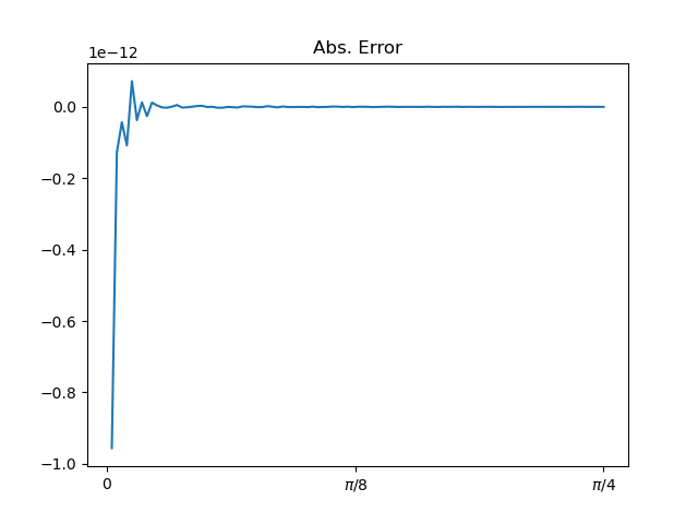
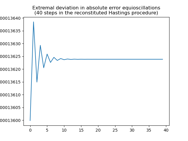
So there is certainly a bit of residual intuitive tweaking in the construction of said polynomials. Moreover a simulation of the Hastings procedure with reasonable parameters: Chebyshev nodes as the starting set of points and all weights set to 1 shows that it converges, rather quickly, to equioscillation with extremal deviation 0.00013718711346827377:
As for relative error, a limit cycle seems to appear:
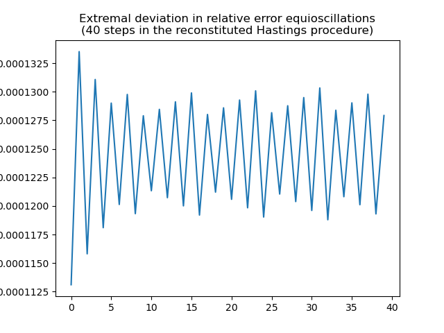
The reconstituted iterative procedure above converges towards the polynomial in the last column of the following table:
| Hastings | Los Alamos | Lagrange Int. | Remez/Sollya | Reconstitution |
|---|---|---|---|---|
| 1.5706268 | 1.5707963 | 1.5706574 | 1.5706597 | 1.5706601 |
| -0.6432292 | -0.6435886 | -0.6434578 | -0.6434767 | - 0.6434802 |
| 0.0727102 | 0.0727923 | 0.0729346 | 0.0729536 | 0.0729563 |
which is closer to the Remez/Sollya-calculated polynomial than to the Hastings polynomial! It appears that applying the procedure described in the theoretical part of the Hastings's book should result into a Remez-like polynomial, such as the one produced by the Sollya system, but instead the slightly different Moon Polynomial is published there.